When you fit a regression model, the intercept is probably not the coefficient you spend the most time thinking about. It represents the baseline response, is usually left unpenalized, and rarely gets much attention in discussions of optimization algorithms. But the way you update this one coefficient can have a substantial effect on how quickly the solver fits the model.
Frederik Fabricius-Bjerre and I study this choice for regularized generalized linear models in our new paper, How to Train Your Intercept: A Comparison of Intercept Update Strategies in Coordinate Descent (Larsson and Fabricius-Bjerre 2026). The code and manuscript source are available on GitHub. Our main finding is that, when the response is imbalanced, a conservative (but common) intercept update can slow down the whole solver. A single Newton step, with a safeguard against overshooting, largely removes this slowdown in our experiments.
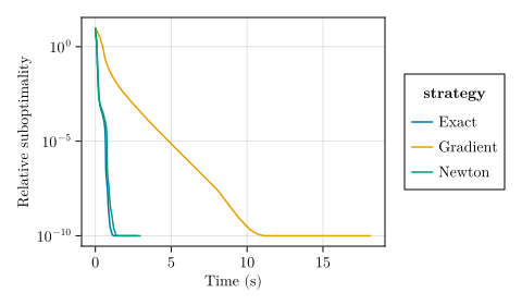
To make this concrete, consider Figure 1. We fit the same regularized logistic regression model to the w1a dataset (Platt 1998) with three strategies for updating the intercept. Everything else in our solver stays the same. The Newton and exact strategies reach the target accuracy after roughly 45 sweeps through all the coefficients. The gradient strategy needs more than seven times as many sweeps.
So, how we update the intercept can make a large difference, but the literature does not examine this choice. My interest in this topic grew when I noticed that implementations of optimization algorithms often differ in how they update the intercept, even though they largely agree on the right way to update every other coefficient. The papers describing these implementations neither explain nor justify their choices.
This led me to propose the problem for a project course in statistics at my department. Frederik was one of the students who chose to work on it. After the course, we continued working together and have now wrapped up the work and submitted the paper to a journal.
The intercept in logistic regression
A logistic regression model describes the probability of a positive response as p_i = \Pr(Y_i = 1 \mid x_i) = \frac{1}{1 + \exp[-(\beta_0 + x_i^\top\beta)]}, where \beta_0 is the intercept and \beta contains the feature coefficients. If all the feature coefficients are zero, the intercept alone determines the predicted probability. For example, a probability of 0.01 corresponds to an intercept of approximately -4.6.
We fit the model by minimizing the logistic loss plus a penalty on \beta, such as the lasso penalty (Tibshirani 1996). The intercept is not penalized. A common way to solve this problem is coordinate descent, which repeatedly updates one coefficient at a time while holding the others fixed.1 We call one sweep over the coefficients a pass. In coordinate descent, the intercept is one of the coordinates, but it has special properties: its update is smooth because it has no penalty, and it remains part of every pass.
1 My earlier work on coordinate descent for SLOPE (Larsson et al. 2023) led me to look into this issue. If you are unfamiliar with coordinate descent, Wright (2015) provides an accessible overview.
Three ways to update the intercept
We compare three strategies, each applied once per pass over the feature coefficients:
- The gradient strategy
- Take one step using a global, worst-case bound on the curvature of the loss.
- The Newton strategy
-
Take one step using the curvature at the current fit.
- The exact strategy
- Minimize the loss over the intercept while holding the feature coefficients fixed.2
2 In the experiments, we solve this subproblem numerically to a tight tolerance.
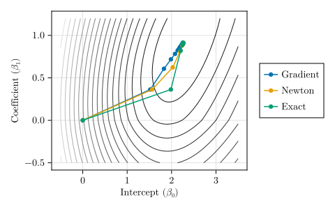
Figure 2 illustrates these choices for a small logistic regression problem with one feature. The curves follow the intercept and feature coefficient as the solver approaches the solution. The gradient strategy takes many small steps, whereas the Newton and exact strategies arrive in only a few.
Why imbalance matters
For logistic regression, the curvature of the averaged loss in the intercept direction is H_{00} = \frac{1}{n}\sum_{i=1}^n p_i(1 - p_i). Since p_i(1 - p_i) is at most 1/4, we can use L_0 = 1/4 as a global curvature bound. If g_0 denotes the derivative of the loss with respect to the intercept, the gradient and full Newton updates are, respectively, \beta_0 \leftarrow \beta_0 - \frac{g_0}{L_0}, \qquad \beta_0 \leftarrow \beta_0 - \frac{g_0}{H_{00}}.
The gradient step is a reasonable choice when the current curvature is close to its upper bound. But when fitted probabilities approach zero or one, p_i(1 - p_i) becomes small, and the two step sizes can differ greatly. In an intercept-only model with a fitted probability of 0.01, the curvature is 0.0099. The full Newton step is then about 25 times as large as the gradient step.3
3 This compares step sizes at the same iterate and does not imply a 25-fold improvement in performance.
Changing the feature coefficients can also change the best intercept value. If the intercept update is too small to keep up, the solver uses that lagging intercept when calculating the next feature updates. The intercept error changes the gradients used for those updates, so a conservative intercept step can slow progress across the whole model.
Doesn’t centering solve this?
If you are familiar with linear regression, you might wonder why we cannot just center the features and separate the intercept from the slopes. For squared loss, that works. The cross-curvature measures how changing the intercept affects the gradient for a feature coefficient. For coefficient j, it is proportional to the mean of feature j. Centering makes that mean zero, so we can optimize the intercept independently of the feature coefficients.
For logistic regression, the corresponding quantity is H_{0j} = \frac{1}{n}\sum_{i=1}^n p_i(1 - p_i)x_{ij}. This is a weighted feature mean. Ordinary centering makes the unweighted mean zero, but generally leaves this weighted mean nonzero. The weights also change as we fit the model. Standardizing the features therefore does not necessarily remove the interaction between the intercept and the slopes.
In me and Jonas Wallin’s earlier work on normalization, we focused on how feature scaling changes regularization (Larsson and Wallin 2025). Centering was simpler: with an unpenalized intercept, we could center the features without changing the fitted model. That remains true for logistic regression, but the computational benefit does not carry over—ordinary centering no longer separates the intercept from the slopes.
How much work should we spend on the intercept?
If a lagging intercept causes trouble, an obvious response is to optimize it fully after every pass. But our experiments suggest that this is usually wasted work. With one safeguarded Newton step per pass, the solver typically follows nearly the same trajectory as with exact intercept minimization, while taking fewer steps to update the intercept. The next sweep over the feature coefficients changes the best intercept value again. Solving for the intercept very accurately before that sweep can therefore waste effort on accuracy that will soon be lost.
The safeguard matters too. Newton’s method approximates the loss near the current fit by a quadratic function and chooses a step using that approximation. If the approximation is poor, the step can be too large and increase the actual loss. We see this in a Poisson example when starting a fit from scratch. A backtracking line search checks each proposed step and shortens it until the loss decreases enough.
What happens in existing solvers?
We also study six production solvers. Some apply coordinate descent directly to the original GLM loss. Others first approximate the loss by a quadratic function, then use coordinate descent to solve that simpler problem.
Within a fixed quadratic approximation, the intercept’s curvature is known, so we can minimize over the intercept directly. But the choice of approximation still matters. An approximation based on the curvature at the current fit adapts to the problem. One based on a worst-case curvature bound can produce the same overly small intercept steps as the gradient strategy.
skglm
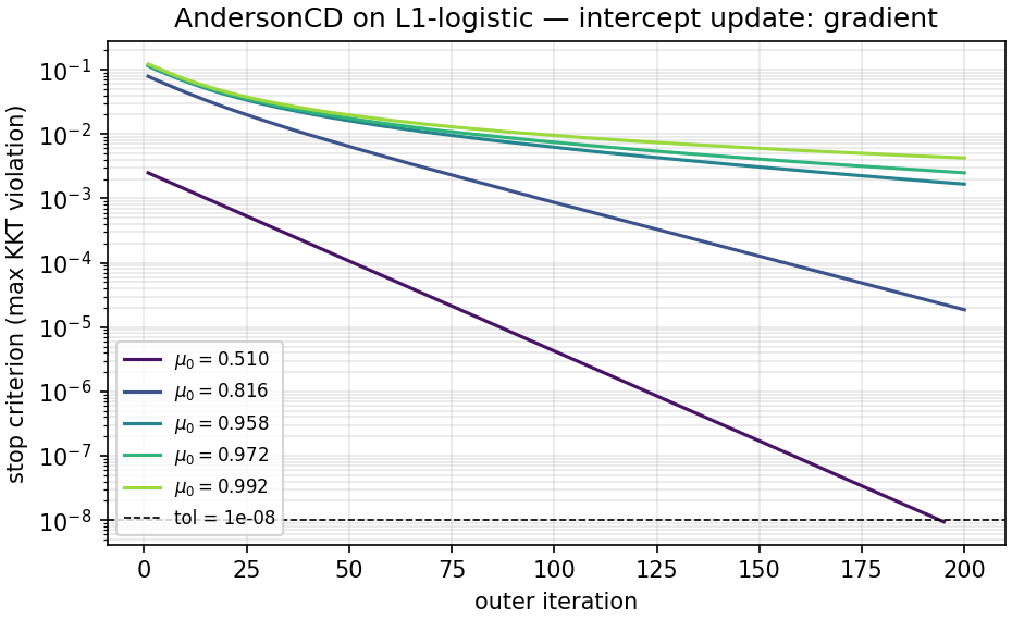
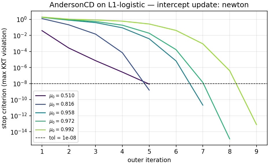
One instructive example comes from skglm. Version 0.5 used a gradient-based update for the intercept. We submitted a patch replacing that update with a Newton step. Figure 3 shows the convergence plots from the PR, where \mu_0 is the fraction of positive responses. With the gradient update, the most imbalanced problems remain far above the stopping tolerance after 200 outer iterations. With Newton updates, all five problems reach tolerance within nine iterations.
Solvers using iteratively reweighted least squares
Solvers such as glmnet (Friedman et al. 2010) use iteratively reweighted least squares (IRLS) to build a local quadratic approximation of the loss. Within each fixed approximation, fitting the intercept is a weighted least squares problem with constant curvature. A single Newton step therefore finds the best intercept value. Using that constant curvature as the gradient strategy’s bound gives the same step, so all three strategies give the same update for this quadratic problem.
These IRLS solvers avoid the slow convergence that we observe in our experiments. I have become more and more convinced that IRLS is the better approach for generalized linear models and have found that it often avoids some convergence traps that direct coordinate descent can fall into.
Conclusion
Our results usually favor one safeguarded Newton intercept update per pass. This simple update avoids the convergence trap of the gradient strategy. Exact intercept minimization requires more work and a more complex implementation, but offers no benefit except in a few edge cases.
Our theoretical explanation is local, and we do not prove a general global convergence rate for coordinate descent with Newton intercept updates. Nevertheless, our analysis and experiments point to the same practical lesson: keeping the intercept in step with the feature coefficients can make a large difference, and doing so often requires only one well-chosen update per pass.